Elemental distribution part 1

We're examining a list of points in which we've accumulated celestial material. The next step is to examine each of the points in turn and determine what elements are going to appear there, and in what concentrations. The basic idea is to distribute the elements according to two parameters: the atomic "weight" of an element and the relative mass of the point we're examining.

The simplest example would be a distribution represented by a diagonal line on a graph where the lightest elements have the highest concentration and the heaviest elements have the least. Like this:

As the elements get heavier, their concentration drops. Easy. This is a line given by f(x) = -x + C (C being some useful offset > 0) and I could give my elements a concentration by simply assigning them a value from that formula with x being the element's number (an analogue for its weight).

But we want to add some more complexity. I'd like that line (without the C factor) to rotate around the origin if the structure were especially heavy, meaning that the concentration of elements in a high-density object would tend towards heavier elements (since more stuff = more pressure = heavier elements created), like this:

And that is just f(x) = x.

So I could say that the elemental concentrations in the least dense object in my galaxy would look like graph #1, and the densest object would look like graph #2. What about everything in between (ie, where most of my points will be)? For example, from these two graphs we would then expect the plot of an object in the exact middle of all densities to look like this:

With every element having a distribution equal to every other element.

Well, I could try performing a matrix rotation on my line based on a given point's density relative to the densest or sparsest points in the galaxy, and then take the integral of the resulting line under the area where the current element would lie, but that would leave me with the difficult problem of expressing the formula of the newly rotated line, and that's not a problem I really want to tackle. Instead, I'll simply use the density of the current point to determine the end-points of my line on the x-axis and then interpolate between those points for each element to get my density (y) values.

Okay, that works nicely, but now what I've got is a bunch of straight lines determining my distributions which is totally unrealistic, so the next step is to introduce some randomness into the concentrations. I will go into this next.

Points of light.

Here's a dump of the history info from my standardized test cell after a test run:

ME value increases for point: [512, 832]
3.6843689007676927E-4
2.716237547371342E-5
2.9090579695712552E-5
3.1144463596306965E-5
6.506629228372208E-5
7.405909856976646E-5
1.7063948094252874E-4
3.3792013449738514E-4
7.444779872999891E-4
0.002446036637268214
0.012186734948650564
0.2634531866962704
0.05472177183706822
----------
ME value increases for point: [512, 132]
3.7562109253996525E-4
2.867135985517093E-5
3.0778210777415476E-5
3.3027122124802656E-5
6.928975898518475E-5
7.921599901756085E-5
1.835023833388631E-4
3.6633310815393274E-4
8.139099483572199E-4
0.00268837270633909
0.01693013582993017
0.3543588907279924
0.04679710557484452
----------
ME value increases for point: [768, 640]
3.760923095653502E-4
2.915072708934144E-5
3.1326436311622165E-5
3.365123867539532E-5
7.064017770270657E-5
8.091135601364832E-5
1.8698489800672439E-4
3.7208456012115634E-4
8.258726661649197E-4
0.002729821637916935
0.01721015128808257
0.40555363904035674
0.09538530622543287
----------
ME value increases for point: [512, 768]
3.767499868527032E-4
2.8279704526428565E-5
3.032241944513951E-5
3.2500398334611576E-5
6.754609983521939E-5
7.69811061138045E-5
1.7632033895116132E-4
3.4639456486021885E-4
7.570867716124853E-4
0.0024541848351469445
0.011871005835509091
0.2395660995876462
0.01219728123002246
----------
ME value increases for point: [0, 640]
3.8561785862321E-4
1.2321449572353496E-5
1.26924945932426E-5
1.3073266099040977E-5
1.3463927338444061E-5
----------
ME value increases for point: [640, 0]
3.722880447846761E-4
9.88352883149037E-6
1.0129457676970466E-5
1.0380636692813959E-5
1.0637132442555548E-5
----------
ME value increases for point: [512, 144]
3.733165328463877E-4
2.750708483139135E-5
2.9457539037267986E-5
3.15347941568521E-5
6.524675689809289E-5
7.416671102236263E-5
1.693333998658301E-4
3.327206820422787E-4
7.26147700986548E-4
0.0023424264101682976
0.01045868543088396
0.02708073563331379
0.0015200371921317774
----------
ME value increases for point: [384, 384]
3.817576409065541E-4
2.9874999870465113E-5
3.212520064006556E-5
6.671118787423355E-5
7.64355917225563E-5
1.7542695358521127E-4
3.4845124474010053E-4
7.711369032722636E-4
0.0025399536635697523
0.0126289164665422
0.26379030752774035
7.561156233093637
158.16191766117714 <---- this point will be something big!
21.97533623061286
2.1882426816866567
1.1442409191569198
0.7480535613845003

I've run tests against my test cell (a cell which generates the same noise map every time) and random cells (random noise maps), and the interesting thing is that, very consistently, one point rises far above the others. This bodes well for the system I've set up, since while the majority of the cells in the galaxy will be "empty" space without significant structure, the ones that do have significant structure will tend to have one high-density point and some variable number of lower-but-variable-density points... just like a solar system. Neat.

Seeds of structure

Now that we've got a list of points that are "dense" enough to spawn structure and some information about how much matter and energy they contain as well as their history, how do we use that information to introduce structure into the local area? This will take me back to what I mentioned earlier about chemistry and fusion of elements. In essence what we have is a whole lot of Element 1 contained in a very small area. We need to take that homogenous soup and turn it into a physical object.

Broad plan:

Step 1: We have to determine, based upon the properties and history of that area, what new elements will form there and how much energy it will take to form them—the idea here being that eventually we will run out of energy to form new elements. The stage/rate at which this happens will produce certain attributes of the eventual structure. The initial density of the area will have a lot to say about that, since a higher density will form heavier elements with less wasted energy.

Step 2: Based upon the elements resulting from Step 1, we determine what sorts of chemical bonding will take place and in what amounts. This refers back to the simple chemistry developed earlier—certain elements will bond with others.

Step 3: The resulting substances from Step 2 will give us an idea of the nature of the structure in question, its chemical composition, size, etc.

One of the biggest kinks to work out here is in the chemistry. Likely I will need to go back and add some more sophistication to that system so that, while elements with the proper "numbers" will bond with certain others, there needs to be some preference in their bonding so that elements will bond in a path-of-least-resistance sort of way.

From clouds to rain

Now, finally, we're getting to the good parts. We have a map of a local area, or cell, with information regarding the amount of matter and energy available to do useful things... but getting from here to there is going to be a lot of work.

The first thing we need is a way to determine A) what elements are present in our cell, B) in what densities and C) at what locations. In order to determine that, we need to know how much energy is required to form elements, so it's back to chemistry.

In the real world, vast amounts of energy in the form of heat and pressure are required to fuse elements—14 million degrees Fahrenheit plus the gravity at the center of a star to fuse two hydrogen atoms together. We're not going to do anything like that here. Instead, we're going to simply use probability ranges to help determine distribution (with, of course, some randomness thrown in) and then the densities present in the local map we already have to determine how much fusion into larger elements will occur.

To simplify things, at least for now, we will first make the decision that we've already expended all the energy necessary to create a galaxy full of the simplest element in our periodic table, meaning that the global and local mass-energy values are what we have left over from that (implicit) process. So instead of just looking at the real universe's elemental abundance and dividing things up based on that, let's just say our entire local map is made up of Element 1. At first.

Now we need to examine the local map very carefully. We need to find concentrations of E1, their constituent values and their areas, which will help us start "fusing" them together into heavier elements. How do we find these concentrations?

To solve this problem, what I've done is created an "accretion algorithm." It's taken me about a month of weekend spare-time work to iterate, evolve and implement. Undoubtedly, I will go back and fine-tune it, but it seems to work well enough to move forward. The idea behind (astrophysical) accretion is the accumulation of celestial matter via the forces of gravity. As more material accumulates, it is able to attract more surrounding material, creating a feedback loop from which, eventually, enough material gathers to form planets, stars, etc. I can't directly simulate this process, not even in two dimensions and not even in a finite problem space—it would take trillions of floating point operations to even begin to see usable results. Instead, I take a few shortcuts using the information I already have in the local cell about where most of the material in the cell will most predictably wind up. After a successful run through (which typically takes a few seconds), roughly 97-99% of the existing material in the cell ends up in the brightest (densest) areas in differing concentrations. This material accumulation takes place in such a way that I record information about it, which will allow me to characterize the different accumulation points--the ones that gathered the most material the quickest could become stars or black holes, while the average areas could become planets, etc.

Sadly, there is nothing compelling, visually, to show for it yet: just a black image with a few white dots here and there. It's the information recorded from the process that will allow me to begin creating celestial bodies—bodies that will not simply be static fixtures, but bodies made of and born from material spawned from an internally-natural and consistent process and which are completely interactive. A gas giant will have harvestable gas. A world of hydrocarbons will have hydrocarbons—usable by anyone who can land there safely and extract it. These will not just be descriptions of static decorations and visual interest. Within the confines of Flat Galaxy, they will be real.

The material density map

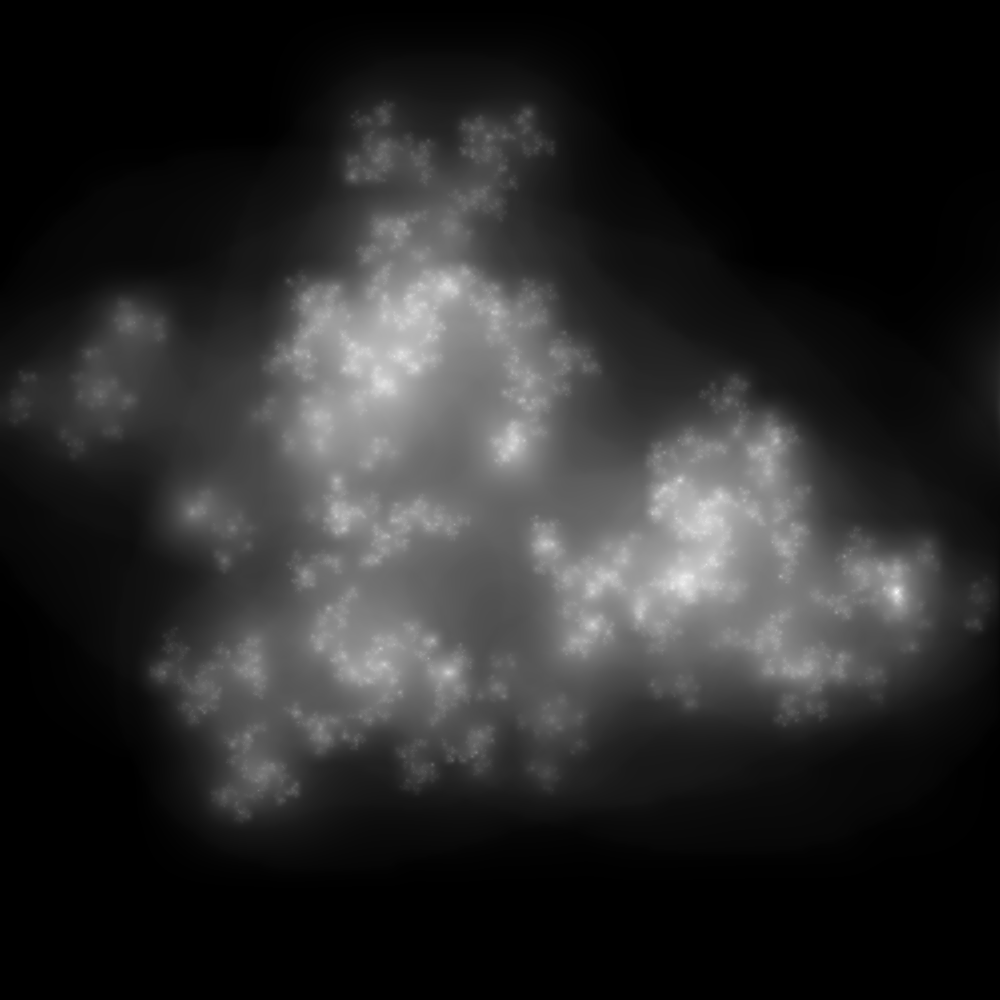
Now we've got something (a fractal-noise image) that reasonably approximates, for our purposes, the elemental-matter-energy density of a galaxy. This would mean that a 1000x1000 pixel image represents an entire galaxy, so if we were making a galaxy the size of the Milky Way each pixel would represent roughly 600 trillion miles or 9.5×10^17 kilometers of space. That's a lot. This is only a proof-of-concept, and I'm not ready to start diving into that kind of scale. I'm going to reduce our galaxy size to something a little more manageable. Let's say about 1/1,000,000,000,000,000th of that size. This is a galaxy about 600 miles or 1000 kilometers across where each pixel represents about 0.6 miles squared (1 km squared). Everything in this galaxy will (probably) be scaled down appropriately: planets, stars, etc.

(Note: I can generate density maps larger than 1000x1000, which would give us much more fine-grained detail about the galaxy, but this is just a starting point. Plus, increasing the size of the image causes pattern generation to take exponentially longer amounts of time and currently results in images that are usually too dim to be very usable. This is something I'll come back to address later.)

Next we need a starting number. This number will be a reference point to the amount of energy and mass that exists in this galaxy (remember they're the same thing both in reality and, very transparently, in our model). We can produce this matter-energy (ME) number by simply totaling the values of each point in our density map. Here's an example number: 32329096.

Now we need to take our density map and divide it up. Each pixel is 1 sq. km, which we need to divide into a bunch of more fine-grained units--basically what will become tiles on a local area map, or cell. A square meter is obviously a good first choice. This means that each pixel on our density map represents a cell of 1 sq. km. * 1000 meters/km = 1,000,000 meters squared. This is a little more than 1/100th of the size of the entire Manhattan area--per pixel, one million times, which means our galaxy is about 1/10th the size of the entire US.

So, say we're examining a pixel in the dead-center of the density map. We can estimate its individual ME value at about 32329096 / (1000*1000) = ~32.33. This small number is the amount of matter and energy we have available to distribute around the cell the pixel on the density map represents. For the time being, we're not going to allow values to distribute across boundaries, so each cell will be in a sense self-contained.

Now the noise functions mentioned in the previous post become really useful. We can generate a 1000x1000 pixel (these represent meters, now) noise map and scale it to our cell's ME value as it relates to the maximum (and minimum) ME values of the entire galaxy, giving us a proportionate and appropriately random (or determined, if we want to direct it a bit) distribution of matter and energy in the cell.

What we need is a noise map that, when we total all its values, equals the local ME value. If our local ME value is 32.33, then we want to produce a noise map where each point's value is, on average, equal to 32.33 / (1000*1000) = 0.00003233. We can do this by producing a random noise map with random values and using a little math to map the values to our desired range. This gives us a noise map with a total ME value equaling its corresponding ME value in the density map. And, if we produce an images from this by normalizing each point in the resulting noise map by the scaled maximum of any point (the density map point with the highest ME value), we can see that each cell has a "brightness" to match:

A cell with 10% of the highest cell's ME value

25%

50%

75%

But herein lies the rub. We can't do this ahead of time, because while each noise map only takes about half a second to produce (that's even using a fast cosine function during interpolation--using the standard Java one takes a second), we're producing one for each pixel on a density map of 1000x1000 pixels. Even if we filter out the pixels with zero values, at least ~50% of the pixels still have a value and it would take about 65 hours to produce every noise map (half that if we use less-pretty linear interpolation--and still far too long). That's apart from the fact that we certainly couldn't hold them all in memory, and they'd eat up about 2 terabytes of HD space. Nope. We need to produce them only as needed. I will begin to address this next.

Blending

I wasn't totally satisfied with the layered fractals being the stepping-off point for a true material density map, so I made some revisions to the code. I spent several days delving into various noise functions and eventually came up with a fairly fast and simple method of blending the disparate-looking fractals using a sort of hybrid Perlin-noise-with-cosine-interpolation function. These are a few of the results:

A lot closer to what I'm looking for. The blending functions aren't perfect and still leave some of the undesired "webbing" between less dense parts of the image, but I can start from here. After basically spending the entire week playing around and with and digging into various noise-generation methods (Perlin, Simplex, midpoint-displacement), I've got a handle on to how to use them going forward for a lot of procedural stuff. Time well spent.

Layered fractals

Per the previous post, here are a few images of layered fractals. Unfortunately, they're not as impressive as I'd hoped as it seems like when one fractal is bright, the other is dim. Rarely if ever are they both bright at the same time. The other problem is that they aren't as organic as I wanted them to be, since using different formulas for each results in images that don't line up nicely and using the same formula for each results in images that look too similar, enough that you often can't tell where one is vs. the other. Nevertheless, they're still pretty cool.

I also made a few more improvements to the fractal generation itself, most notably introducing multi-threading logic to the (embarrassingly parallel) pattern generation so that generating ten two-fractal images went from taking about 50 seconds on average to taking just 20 seconds on average. I'll take a 60% speed improvement anytime.

(Edit: I forgot to apply my previous optimization for those numbers. With both of my optimizations, the multi-threaded version takes 10 seconds to generate 10 two-fractal images while the one-thread version takes 30 seconds. With none of my optimizations, that same set took about 50 seconds to generate, a total improvement of about 80%).

And here's a couple single-fractal images I just thought were really awesome.